Exposing to the right (“ETTR”) is, in some circles, a pretty contentious issue—in part because there have been a number of slightly misleading articles on the subject, which have themselves led to rebuttals which sometimes only add to the confusion. Its origins stem from an article published in 2003 by Michael Reichmann on his website Luminous Landscapes following a conversation with Thomas Knoll, a former lead developer on Photoshop.
So what is it? It is the practice of over-exposing a scene so that the image reaches, but doesn’t pass, the right-hand side of the histogram and then bringing the exposure back down in post-editing so that the image is correctly exposed.
The reason that ETTR can, in some cases, produce a higher quality image is two-fold:
- (The main reason). By over-exposing and thus shifting the image to the right-hand side of the histogram you are increasing the signal-to-noise ratio (more signal, same noise = higher signal-to-noise ratio).
- (The lesser reason). Relative to the shadows, we see finer transitions between tones in the highlights, therefore capturing images using the brighter regions of the histogram gives us a final image with more tones.
The above reasons only truly hold if you are (1) shooting in RAW (adjusting exposure on a JPEG using post-editing software is a destructive process), and (2) shooting at ISO 100 (if you can over-expose at ISO 200 and still not clip the image it means you can also drop down an ISO which would be a better option to reduce noise). Let’s look at each of these individually.
Signal-to-noise ratio (SNR)
This is pretty self-explanatory and the reasons why a lower ISO gives a better signal-to-noise ratio and thus a higher image quality has been detailed in the article on noise. But by way of a brief explanation, the electric charge produced by each pixel is amplified before it is turned into a analogue-to-digital unit (ADU). Higher ISOs are amplified more (because less light has been collected), but this process also amplifies noise leading to a lower image quality.
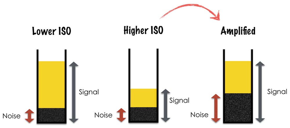
By increasing the exposure time and pushing the histogram to the right (without clipping) you are increasing the overall signal (number of photons collected) and reducing the signal-to-noise ratio.
Finer Tonal Transitions
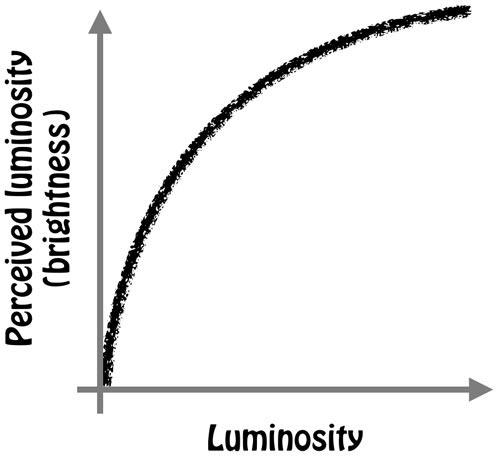
Camera sensors are linear devices. The digitized value they spit out for each pixel is directly proportional to the number of photons that hit the photodiode. If you double the light intensity or luminosity, the output value will also double. Human vision, on the other hand, is non-linear. We are far more sensitive to changes in low-light than we are to changes in well-lit conditions. The relation between actual luminosity and our perception of luminosity is reasonably estimated by the below graph.
Consequently, if we were to view the linear output of the camera’s dynamic range—in other words, from black to white and every incremental step in between—this is what we would see:

Whereas, intuitively, we would expect to see something more like this:

The number of “levels” between black and white depends upon the camera’s bit depth. Bit depth is independent of dynamic range. Dynamic range, typically measured in f-stops, is the range outside which the camera only records white or black. If dynamic range is distance, then bit depth is the units used to divide up the distance—and no matter what the unit (millimeters, inches, metres) the start and end points are always the same: black and white. And no matter what units you use to divide the distance, the distance between black and white is the same (10 kilometres = 10,000 metres = 1,000,000 cm = etc.).
As I’ve stated elsewhere, histograms are gamma-encoded. The distribution between black and white is much more closely aligned with the lower gradient bar than the upper (the “camera sensor” view). But let’s, for the sake of explanation, unencode our histogram so that the gradient distribution follows the linear pattern of the camera sensor. This is easily done since gamma-encoding just applies an exponent to the tonal value and reversing it is just a simple mathematical process (which cameras, computers and LCD monitors do all the time).
For the unencoded, linear histogram we can divide it up into equal levels—the number of which depend on the bit depth of the camera (okay, most histograms are shown on an 8-bit or 256-level basis regardless of the bit depth of the camera, but since I’m already making up my own histogram allow me this liberty—it doesn’t change the argument, in any case). Let’s assume we’re using a 8-bit camera (so 256 levels) with a dynamic range of 6 stops. We know two things:
- The 256 levels are evenly split over our unencoded histogram.
- Which each stop down the amount of light hitting the sensor is halved.
So going from black to white we have a gradient line at the bottom of our histogram that looks like this:
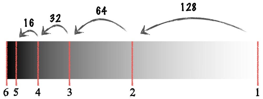 Consequently, we can see that half the data is actually included in the 1st stop and if our unencoded histogram doesn’t stretch into this section then we will only be working with half of the available data. By exposing to the right we ensure that we utilize this data meaning that when the image is finally gamma-encoded we have finer transitions between the levels.
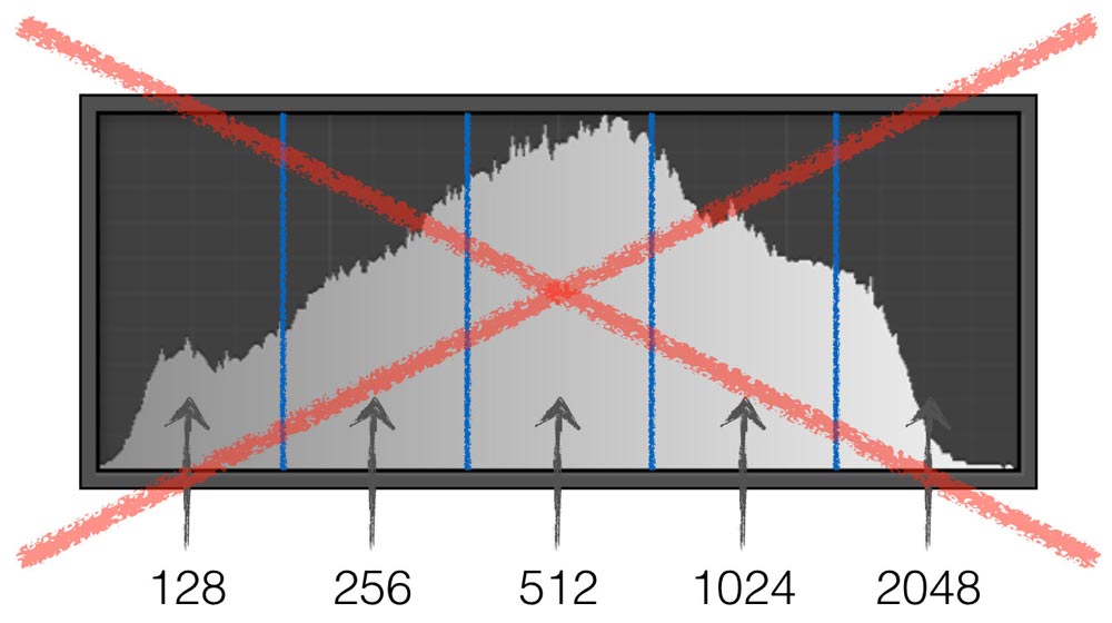
It’s worth pointing out that most of the confusion around ETTR comes from either not realising that bit depth has nothing to do with dynamic range or, more commonly, not realising that the histogram we see on our camera’s LCD display or in our post-editing software is gamma-encoded. The latter misunderstanding leads to the following bit of sophistry (example for a 12-bit camera).
But does it actually work?
Some say yes, others say no. The theory is certainly solid but, practically speaking, the advantages are questionable. Firstly, in your bid to push the histogram as far to the right as possible you’ll be working with the jpeg version of the RAW file used to produce the histogram you see on your camera LCD—and this might only be a close representation of the final histogram once you’re back working the RAW file with your post-editing software. Especially if you’re viewing the RGB or luminosity histogram (which most would be) then it won’t reveal clipping in an individual colour channel. All of this means that you’re more likely to inadvertently clip the image in your bid to get the highest signal-to-noise ratio; and if you clip the image then detail is lost for ever.
Ultimately, is the risk worth the reward? Given that you need to be shooting at ISO 100 on a high quality camera (I’m going to assume you’re not reading this article to expose to the right on a point-and-shoot…) to yield any potential benefit then is noise going to be so much of an issue that you want to risk clipping an individual colour channel? I would argue not—and as image sensors improve the reasons for exposing to the right diminish exponentially.